Saturn Rings Point Generation
Generate a rib archive containing point clouds coordinates and color data for Saturn Rings using Python. The rib archive is then rendered in Renderman in Autodesk Maya.
The project began with Professor Malcom Kesson’s writeRing function.
Researching Saturn Rings Data
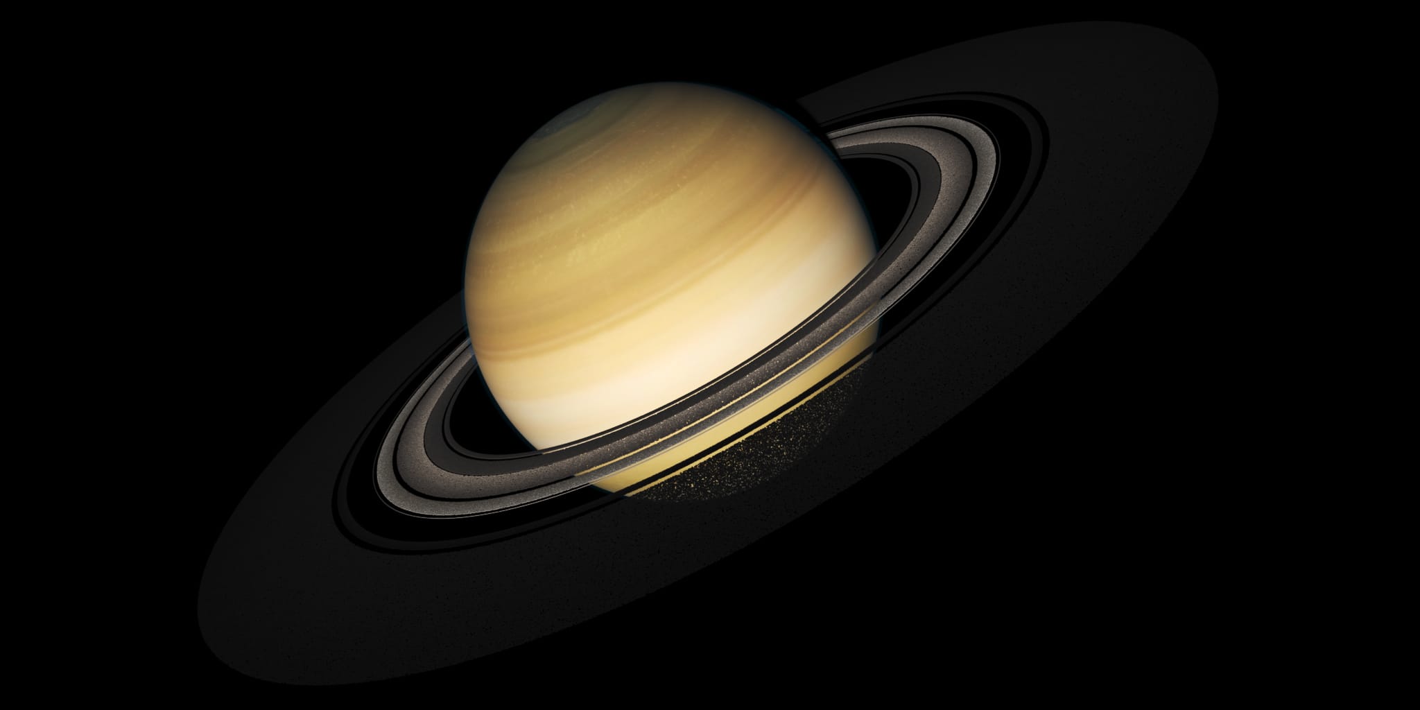
Before diving into the code, it was essential to learn more about Saturn and its rings since it has a singular objective form in our world. In my research, I discovered that Saturn has 7 rings with their own respective radii. There are many data available online: NASA, TIVAS, but the one I consulted was Britannica.
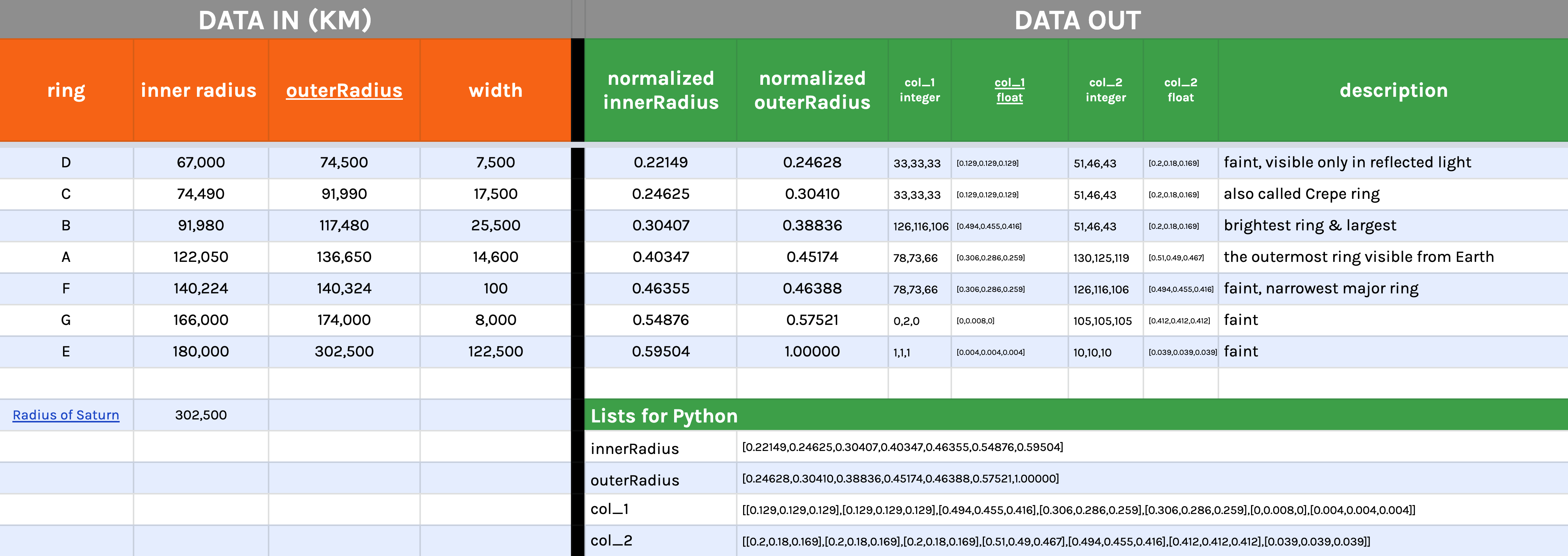
Using Google Sheets and formulas, I normalized the inner and outer radii of each ring by dividing them with the whole planet’s radius. I also added the different colors from the rings into this database. From there, I generate lists/arrays that I can use in my Python functions.
Generating the rings
The way I wrote my function is to avoid writing multiple writeRing 7 times, I wanted to do that with a for-loop, and have the ability to change the radius without having to change each individual rings’s radii. Hence, that is why I used lists of normalized ratio instead. I also created lists for the start and end colors for each ring.
					# rib_particles.py / writeSaturnRings

def writeSaturnRings(path, s1, s2):
    # normalize ring values where r1 = innerRadius, r2 = outerRadius
    r1 = [0.00, 0.25, 0.30, 0.40, 0.46, 0.55, 0.60]
    r2 = [0.25, 0.30, 0.39, 0.45, 0.55, 0.58, 1]
    pts = [0.7, 0.7, 1, 1, 1, 1, 3]

    # color
    col_1 = [[0.129, 0.129, 0.129], [0.129, 0.129, 0.129], [0.494, 0.455, 0.416], [
        0.306, 0.286, 0.259], [0.306, 0.286, 0.259], [0.000, 0.008, 0.000], [0.000, 0.008, 0.000]]
    col_2 = [[0.200, 0.180, 0.169], [0.200, 0.180, 0.169], [0.200, 0.180, 0.169], [
        0.510, 0.490, 0.467], [0.494, 0.455, 0.416], [0.149, 0.149, 0.129], [0.149, 0.149, 0.129]]

    numRings = len(r1)

    for i in range(numRings):
        inner = r1[i] * s2 + s1
        outer = r2[i] * s2 + s1
        myPts = pts[i] * 20000
        newPath = path + '_ring_' + str(i + 1) + '.rib'
        writeRing(newPath, myPts, inner, outer, .1, col_1[i], col_2[i])

    # write rib that reads all ribs created
    # writeReadArchive(path, '_ring_', numRings)
Rib to read rib archives
Also, just to challenge my comprehension of Python, I wrote a function that generate a rib archive that writes all the directories of the rib archives that was generated from above function. It runs a loop statement based on the number of rings specified. In this case, there are seven of them, and my function appends the rib name with counter variable and a line break.
					# rib_particles.py / writeReadArchive

def writeReadArchive(path, rib_name, num):
    rib_file = open(path+'_rings.rib', 'w')
    rib_file.write('##bbox: -50.000000 -0.000000 -50.000000 50.000000 0.000000\n\n')
    for i in range(num):
        rib_file.write('ReadArchive ' + '"' + path + rib_name + str(i+1)+'.rib"\n')
    rib_file.close
OUTPUT
					##bbox: -50.000000 -0.000000 -50.000000 50.000000 0.000000

ReadArchive "/Users/ddu/Desktop/vsfx705/classwork/data_ring_1.rib"
ReadArchive "/Users/ddu/Desktop/vsfx705/classwork/data_ring_2.rib"
ReadArchive "/Users/ddu/Desktop/vsfx705/classwork/data_ring_3.rib"
ReadArchive "/Users/ddu/Desktop/vsfx705/classwork/data_ring_4.rib"
ReadArchive "/Users/ddu/Desktop/vsfx705/classwork/data_ring_5.rib"
ReadArchive "/Users/ddu/Desktop/vsfx705/classwork/data_ring_6.rib"
ReadArchive "/Users/ddu/Desktop/vsfx705/classwork/data_ring_7.rib"
NORMALIZING DATA WITHIN Python
One mistake that I discovered with the previous method of normalizing the values in Google Sheet is that I do not get the full float values of the data since I rounded them to 5 decimals place. Optimally, I should have prepared the radii data as it is in a CSV format which then can be opened and read in Python. A similar improvement that I made was to write a function that normalizes the values in an array based on the max value input as shown below. This way, I can normalize not just the radii but also the RGB integer values into float (0-1) thus ensuring precision with less human errors of inputing wrong values.
* One thing I also learned about Python regarding float values is that your numbers need have a decimal point in order to calculate float values. For example, 33÷255 will yield 0, but 33.0÷255 will yield 0.129…
					def normalizeValues(arr,maxValue):
    #arr must have at least one decimal to print float values
    normalized = []
    for i in range(len(arr)):
        normalized.append(arr[i]/maxValue)
    return normalized

normalizeValues([29,200,30],255.0) # RGB float
REVISED WRITE FUNCTION
					# rib_particles.py / writeSaturnRings

def writeSaturnRings(path, s1, s2):
    # normalize ring values where r1 = innerRadius, r2 = outerRadius
    r1 = [0.00, 0.25, 0.30, 0.40, 0.46, 0.55, 0.60]
    r2 = [0.25, 0.30, 0.39, 0.45, 0.55, 0.58, 1]
    pts = [0.7, 0.7, 1, 1, 1, 1, 3]

    # color
    col_1 = [[0.129, 0.129, 0.129], [0.129, 0.129, 0.129], [0.494, 0.455, 0.416], [
        0.306, 0.286, 0.259], [0.306, 0.286, 0.259], [0.000, 0.008, 0.000], [0.000, 0.008, 0.000]]
    col_2 = [[0.200, 0.180, 0.169], [0.200, 0.180, 0.169], [0.200, 0.180, 0.169], [
        0.510, 0.490, 0.467], [0.494, 0.455, 0.416], [0.149, 0.149, 0.129], [0.149, 0.149, 0.129]]

    numRings = len(r1)

    for i in range(numRings):
        inner = r1[i] * s2 + s1
        outer = r2[i] * s2 + s1
        myPts = pts[i] * 20000
        newPath = path + '_ring_' + str(i + 1) + '.rib'
        writeRing(newPath, myPts, inner, outer, .1, col_1[i], col_2[i])

    # write rib that reads all ribs created
    # writeReadArchive(path, '_ring_', numRings)
Generating Maya nParticles
Having learn how to write functions and modules to generate rib archive, the next step was to generate particles using the script editor with Maya. The same concept of using the gen_points module still applies, but this time the data could be fed directly into the nParticle coordinates. Below is the new Python module “nParticle.py” that does that and the Python code to input in the Script Editor .
*Ensure that your python scripts are in Maya script folder for the Script Editor to use them.
					// nParticles.py

import gen_points
import math
import maya.cmds as cmds


def writeCubic(num, side):
    data = gen_points.cubic(num, side)
    cmds.nParticle(p=data)


def writeBox(num, width, height, depth):
    data = gen_points.box(num, width, height, depth)
    cmds.nParticle(p=data)


def writeSpherical(num, radius):
    data = gen_points.spherical_kesson(num, radius)
    cmds.nParticle(p=data)
MAYA SCRIPT EDITOR
					import nParticle
reload(nParticle)

nParticle.writeSpherical(200,5)
nParticle.writeCubic(200,4)
nParticle.writeBox(200,10,4,0.2)
RENDERS + USING FIELDS
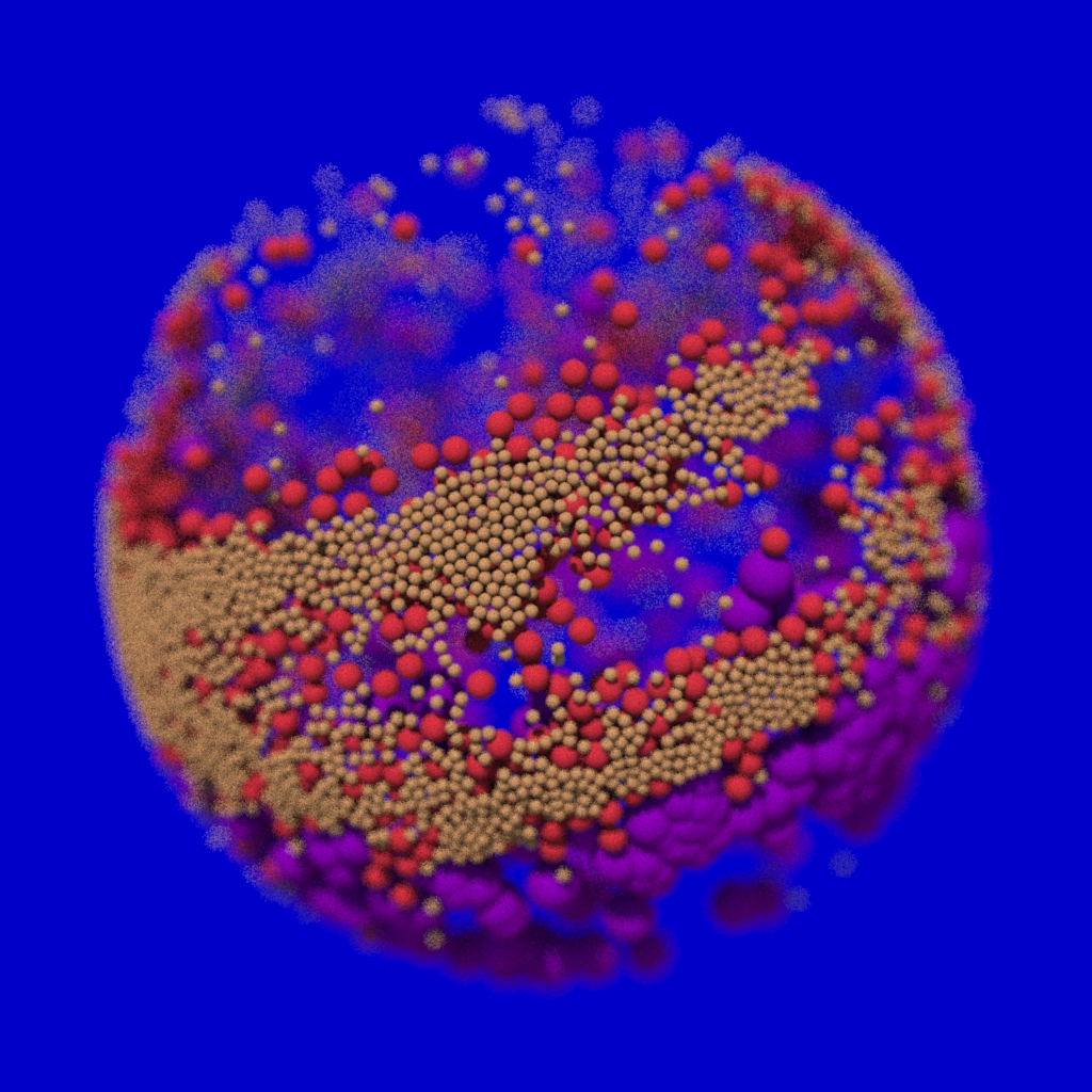
Aside from a Python study, I also got to investigate how to utilize Fields to create interesting design and motion. For the 1st video above, the primary Field that I used was a Radial Field which made all the spheres squished together, and since self-collision was turned on, the form is always in flux. In addition, I added a Vortex and Turbulence Fields to add secondary motion and make it look more organic.
As for the 2nd iteration, I used two spheres as passive colliders and filled the space in between them with nParticles, and used the same set of fields with different settings. I got lots of interesting results from this experiment, below are the most pleasing variants I created.


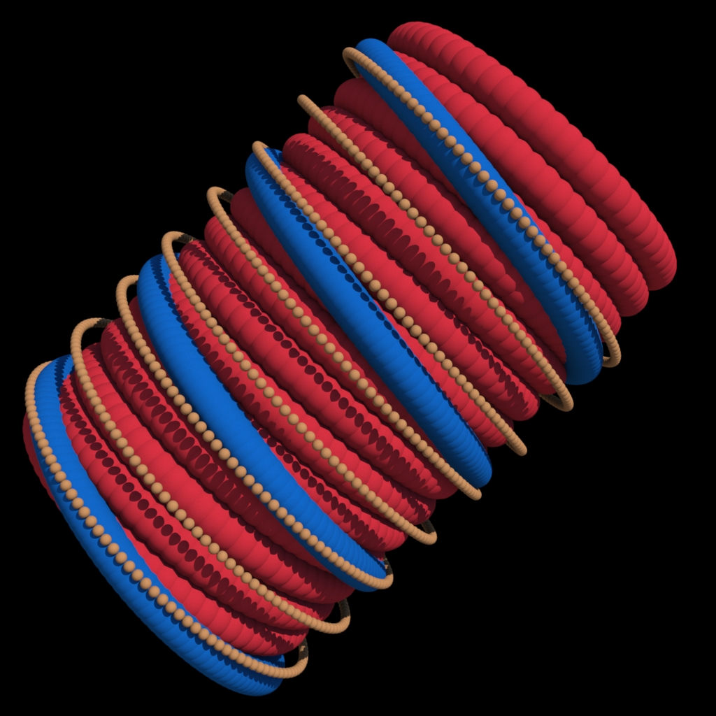
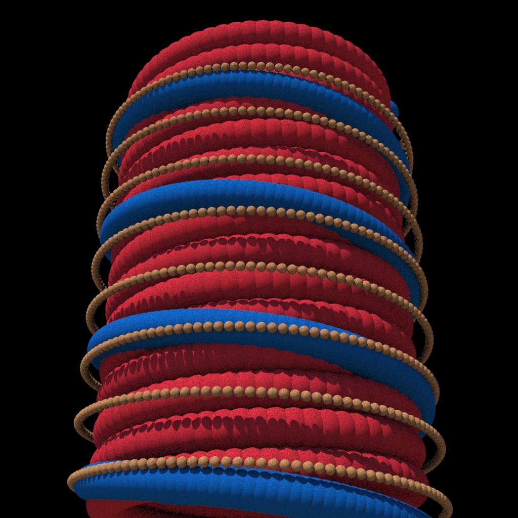
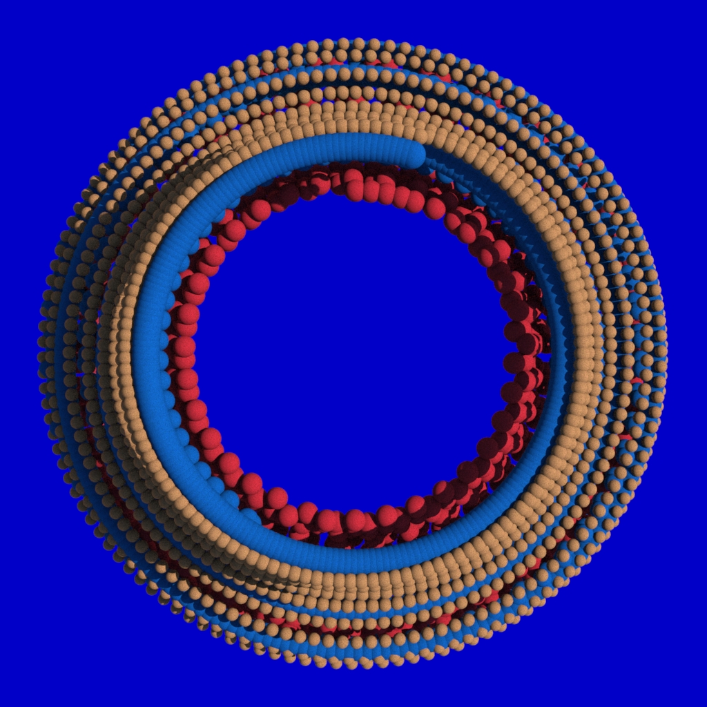
Finally, to wrap up this whole study, I wrote another function in gen_points.py to generate spiral particles in Maya and implement the nParticles
					// gen_points.py / helix

def helix(num, radius, height, freq):
    data = []
    n = 0

    while n < num:
        #theta = n/num
        n = float(n+1)
        theta = float(n/num*2*math.pi)
        x = radius * math.cos(theta*freq)  # math.cos(theta)
        z = radius * math.sin(theta*freq)  # math.cos(theta)
        y = height * (n/num)  # math.sin(theta)
        # x = random.uniform(-radius / 2, radius / 2)
        # y = random.uniform(-radius / 2, radius / 2)
        # z = random.uniform(-radius / 2, radius / 2)
        data.append((x, y, z))
        n = n + 1

    return data


// nParticle.py
    def writeHelix(num, radius, height, freq):
        data = gen_points.helix(num, radius, height, freq)
        cmds.nParticle(p=data)
Conclusion
Python is pretty neat. Though this assignment was fairly simple, I learned a lot just by thinking about how to generate point clouds in different geometric forms. In addition, I got more comfortable with Maya which I have dreaded for the past decade.
Anyway, I look forward to see how this knowledge can be incorporated into Motion Design and other VFX tools!
